Example: PTSD Assessment

library(tidyverse)
library(tapModel)
library(LaplacesDemon) # for mode and rbern
library(knitr)
library(kableExtra)

set.seed(1234)

ratings <- tapModel::generate_sample_ratings(N_s = 200, N_r = 10,
                                             params = list(t = .5, a = .65, p = .8),
                                             details = TRUE)

1 Example: Uniform Raters

As a simple illustration of model assessment, I’ll start with a simulated data set where all the raters and subjects have the same average parameters, subject only to sampling error. The data set is generated with 600 subjects and 10 raters each (the same as the ptsd data, which we’ll consider next), with \(t = .5\), \(a = .7\), and \(p = .2\). The raters are significantly biased away from Class 1. One purpose of this example is to inspire some confidence in the method, since we already know the parameter values. Another purpose is to show how we can investigate a parameter set by simulating values from it to make sure we can recover them. This can be done, for example, after estimating parameters from a real rating set.

2 Are the estimated parameters reasonable?

Here, we know the real values of the parameters, so our expectations are exact. We can compute the three-parameter model with the functions provided in the tapModel package.

params <- tapModel::fit_counts(as_counts(ratings))

params |> 
  select(t, a, p) |> 
  kable(digits = 2) |> 
  kable_styling(
    full_width = FALSE,           # <- stops spanning the full page
    position   = "center",
    bootstrap_options = c("striped","hover","condensed")
  )

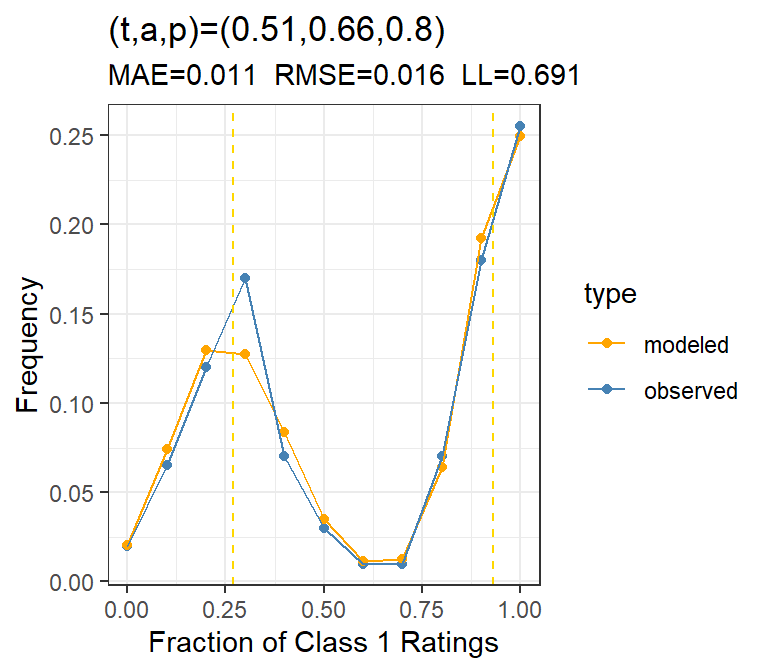
Table 1: Model fit for 20 uniform raters on 200 subjects, showing the fitted parameters for the average t-a-p model with simulated ratings where t = .5, a = .65, and p = .8.

t	a	p
0.51	0.66	0.8

The parameters don’t look degenerate (close to zero or one).

ratings |> 
  as_rating_params(params) |> 
  subject_calibration()

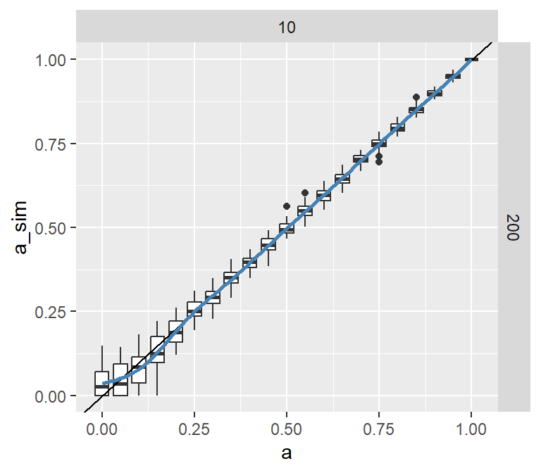
Figure 1: Subject calibration for the three-parameter model.

3 Where is the DK Horizon?

The next step is to find the Dunning-Kruger threshold for this data configuration. Recall that this is a reframing of the null hypothesis \(p\)-value to emphasize ignorance.

tapModel::simulate_exact_fit(200,10,n_sim = 50, output = "plot")

Figure 2: Ranges of accuracy estimates for nominal t = p = .5 samples.

The boxplots in Figure 2 show that the DK-horizon is low, maybe around \(a=.15\) as the point past which we can’t trust accuracy estimates. If we want, we can put numbers to this by simulating \(a=0\) to see how large the accuracy estimates can be from sampling error.

dk <- dk_horizon(200, 10, n_sim = 200)
dk |> 
  as.tibble() |>  
  mutate(Threshold = names(dk)) |> 
  select(Threshold , Accuracy = value) |> 
  kable(digits = 2) |> 
  kable_styling(
    full_width = FALSE,           # <- stops spanning the full page
    position   = "center",
    bootstrap_options = c("striped","hover","condensed")
  )

Table 2: Estimated percentiles for accuracy, given 200 subjects with ten raters each, when accuracy is actually zero.

Threshold	Accuracy
50%	0.00
75%	0.08
90%	0.11
95%	0.13
98%	0.15

For a data set of this size, 98% of the randomly generated ratings resulted in an accuracy parameter estimate of .15 or less. It’s reasonable to be suspicious of parameter estimates that have \(a\) below that threshold. We might be being fooled by sampling and estimation error into thinking the raters are much more accurate than they actually are. In this case, with an estimate of about .65 (the true value), we easily pass the DK-threshold test.

4 Do we need a hierarchical model?

Next we assess the likelihood in units of bits/rating to compare the three-parameter model to the more detailed hierarchical model.

rating_params <- tapModel::fit_ratings(ratings)

subject_calibration(rating_params)

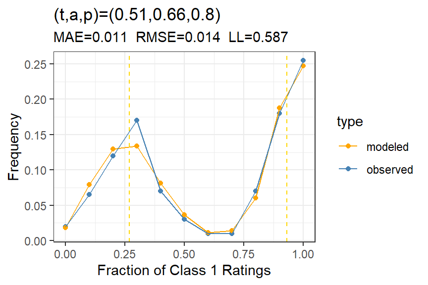
Figure 3: Model fit for uniform raters, showing the simulated distribution of bits per rating for the average and hierarchical t-a-p models with simulated ratings where t = .5, a = .7, and p = .2. The vertical lines shows the bits per rating for each model with the original data set, and the densities are for data sets simulated from the respective parameters.

The model fit in Figure 3 shows overlapping distributions of log likelihoods for the hierarchical and average (three-parameter) t-a-p models. Recall that better fit for a model means a smaller value of bits/rating (hence larger likelihood). Here there’s no difference between the two models, so we can conclude that the hierarchical model is adding parameters with no benefit. In this case, we would choose the average three-parameter t-a-p model as the most parsimonious description of the data. Because this is simulated data, we know that’s the correct conclusion.

5 Independence

range <- rater_cov_quantile(rating_params) 
cov_results <- rater_cov(rating_params)
plot_rater_cov(cov_results, range)

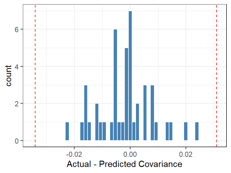
Figure 4: Distribution of actual - expected covariance between raters, with 96% confidence interval marked.

There doesn’t seem to be an issue with independence, at least as far as correlations can assess. This isn’t surprising, since we know how the ratings were created.

6 Summary

For this example, we already knew the parameter specification, and the goodness-of-fit process confirmed that the estimate was probably trustable. Moreover, it confirmed that there’s no advantage to choosing a more complicated hierarchical model.

I chose the sample size and t-a-p parameters for this example because they also correspond to the PTSD data’s specifications. You might refer to that example for more.